Surveillance

Companion

Analysis

Companion session to the surveillance Fetch-R module

Objectives

Reuse skills aquired in the FETCH-R modules (import, clean and visualize data)
More specifically, analyze surveillance data to detect alerts and to help decide which alerts to prioritize for further field investigation.

Introduction

Warning. This session is a companion to the case study Measles emergency response in the Katanga region (DRC) from the FETCH Surveillance module and might not make sense as a standalone tutorial.

From an R point of view, this tutorial builds on skills acquired throughout the FETCH-R modules, introduces a couple of useful generalist functions, and some more specialized ones.

Tip

Do not hesitate to refer to past sessions and your own scripts to remind yourself of some functions!

Setup (Question 2)

Since this is part of a specific module, you will create a new RStudio project. We refer you to the main session for help creating a project and importing your data.

Setup a new project

Create a folder surveillance_case_study associated with the FETCH Surveillance module. Add the following subfolders in it:

📁 data
- 📁 clean
- 📁 raw
📁 R
📁 outputs

Create an RStudio project at the root of the surveillance_case_study folder.
If you do not already have the data from the case study download them.

4. Unzip the archive if you just downloaded. Save the two Excel files in the subfolder data/raw.
5. Create a new script called import_clean.R and save it in the R subdirectory. Add metadata and a section to load the following packages: {here}, {rio}, and {tidyverse}.

Import data in R

Reminder from the case study: you requested access to the routine surveillance data and the laboratory data to the DRC MoH. The MoH agreed to share it with you on a weekly basis. The first dataset you received is of week 20 in 2022 (the data we are working on are simulated).

If you have not done it already, open the raw data files in Excel (or another equivalent application) to inspect them.

The surveillance dataset is pretty straightforward to import. The lab dataset is slightly trickier: the data headers do not start at line one. Fear not, the skip argument from the import() function is made for this situation:

# DO NOT RUN (PSEUDO-CODE)
import(
  here("data", "raw", "example_file.xlsx"), 
  skip = 3  # Skip the first three lines and start importing from line four.
)

Add a section to your script dedicated to data importation.
Import the surveillance data and store it into a data_surv_raw data frame. Then, import the lab data and save it in a data_lab_raw data frame.
Verify that the import went well for both data frames (Viewer, check the dimensions or start and tail of data frames).

Cleaning (Question 2 and 3)

Surveillance data (Q2)

Now that the data is correctly imported, we are going to perform some more checks, as usual, before a bit of cleaning.

Quick checks

During the case study you won’t have time to inspect and clean all columns within the available time, so for now we will focus on key columns: health_zone, week, totalcases and totaldeaths.

Note

If you work on this tutorial in your own time, inspect the quality of the other columns and cross-check information of several columns. We refer you to the discussion of the case study for more checks to perform.

Add a section for the exploration and cleaning of the surveillance data into your script.
Now, explore the surveillance data frame and answer the following questions:

What are the column names?
How many provinces are in the dataset? Is this coherent with what you expect?
How many health zones are in the dataset?
What is the range of weeks?
What is the min of totalcases?
What is the max of the totaldeaths?
Do you notice missing data for these columns? Are the strings of text clean?

Clean strings

Now that we have a better idea of what is the state of the data, let’s start cleaning. We are going to write a cleaning pipeline like we did in the main modules (check out your code for the end of the cleaning modules to see an example final pipeline).

Tip

To facilitate debugging your pipeline, add commands one by one, checking each new command before adding a new one.

We are going to perform a couple of actions on the columns containing text to remove potential problems:

transform them to lower case
remove potential extra spaces
replace - and spaces by _.

Because you may not have the time to do all of text colums, work on the health_zone or the province column for the following instructions.

Start a cleaning pipeline with a mutate() that turns the chosen column to lower case.

Now, we are going to introduce two handy functions for more text cleaning. The first one is the str_squish() function from the {stringr} package (help page here), that removes spaces at the start or end of the strings, and replace multiple spaces in the middle of a string by a single space.

examples <- c(" Trailing spaces     ",
              "Multiple     spaces",
              " Everything     here ")

str_squish(examples)

[1] "Trailing spaces" "Multiple spaces" "Everything here"

The other function, str_replace (also from the {stringr} package) does what you expect from its name: replace something in a string by something else. It has a pattern argument that take the bit of text to be replaced, and a replacement arguments that takes the bit of text to use as replacement:

str_replace(
  "HAUT-KATANGA",    # A string of text (or a column, if used in a mutate)
  pattern = "-",     # The bit to replace
  replacement = "_"  # The replacement
)

[1] "HAUT_KATANGA"

Add steps to your mutate to:

Remove all unwanted spaces from your chosen column
Change the - and to _ in the column (in two steps)

The head of these columns should now be:

  country     province    health_zone disease
1     drc haut_katanga mufunga_sampwe measles
2     drc haut_katanga        sakania measles
3     drc haut_katanga        mitwaba measles
4     drc haut_katanga kilela_balanda measles
5     drc haut_katanga         likasi measles
6     drc haut_katanga         kikula measles

Store the result data frame in a data_surv object.

Save the clean data

Use the {rio} package to export data_surv to a .rds file called data_ids_2022-w20_clean in the data/clean subfolder of your project.

Laboratory data (Q2)

We are going to follow the same steps as before for the lab data, and focus for now on the columns health_zone, igm_measles and igm_rubella.

Quick checks

Perform data checks on the colums names and dimensions. What are the categories for igm_measles and igm_rubella? What do you need to do to clean these columns?

Clean and recode strings

Start a new cleaning pipeline to clean the lab data. As before, for one of the text column, change it to lower case, remove the extra spaces and replace the or - by _.
Recode at least one of igm_measles or igm_rubella columns so that the categories are negatif, positif and indetermine.
Store the cleaner version in a data_lab data frame

The head of the cleaned columns should now be:

   health_zone igm_measles igm_rubella
1      kambove    negative    negative
2      kambove    negative    negative
3      kambove    negative    positive
4      kambove    negative    negative
5      kambove    negative    positive
6      kambove    negative    negative
7      kambove    negative    negative
8      kambove    negative    positive
9       manika    negative    negative
10   kamalondo    negative    negative

Tip

You can use the case_when() function to recode the IGM columns.

Save the clean data

Export the data_lab data frame to a .rds file called data_lab_2022-w20_clean in the data/clean subfolder of your project.

Going further

This is the end of the steps for question 2! If you finished in advance and there is still time, reuse the functions we just saw to clean the other text columns in both datasets and recode both IGM column in the lab dataset.

If you still have time, perform more checks on the data:

Display the health zone for which the numbers by age group add up to a different number than the total (if any)
Are there any health zone for which the number of deaths is higher than the total number of cases?
Are there duplicated lines (fully duplicated, or several values for health zone and week)?
Are there unrealistic case numbers?

Complete surveillance dataset (Q3)

During the case study and the data checks, you realized that some weeks are missing from the surveillance dataset. You discussed the possible reasons for it, and the associated problems. Here we are going providing code to create a dataset that contains all weeks (assuming that missing weeks had zero cases and deaths).

We will use the function complete() from the {tidyr} package to add the missing lines and fill the columns containing numbers (totalcases and totaldeaths) with zeros. Due to the constrained time, we will give you the code for now, but check out the details in the Going further section when you have time.

Start a new pipeline that takes the data_surv data frame and keeps only the columns province, health_zone, week and total cas.
Add a new step to your pipeline and paste the following code to complete the data frame:

complete(
  # Use all the existing combinaitions of province and health zone:
  nesting(province, health_zone),
  
  # All the combinations whould have all weeks from the minimum (1) to the maximum (20) of the week column.
  week = seq(min(week, na.rm = TRUE), 
             max(week, na.rm = TRUE)),
  
  # Fill these two columns with zeros for the newly created weeks:
  fill = list(totalcases  = 0,  
              totaldeaths = 0 
  )
)

Store the result of the pipeline in a data frame called data_surv_weeks. The head of that data frame looks like:

# A tibble: 10 × 5
   province     health_zone  week totalcases totaldeaths
   <chr>        <chr>       <dbl>      <dbl>       <dbl>
 1 haut_katanga kafubu          1          0           0
 2 haut_katanga kafubu          2          0           0
 3 haut_katanga kafubu          3          0           0
 4 haut_katanga kafubu          4          0           0
 5 haut_katanga kafubu          5          0           0
 6 haut_katanga kafubu          6          0           0
 7 haut_katanga kafubu          7          0           0
 8 haut_katanga kafubu          8          0           0
 9 haut_katanga kafubu          9          0           0
10 haut_katanga kafubu         10          0           0

When you are done, export that data frame to a .rds file called data_ids_2022-w20__weeks_clean in the data/clean subfolder of your project.

Going further

This is the end of question 3; if you are finished in advance, do not hesitate to carry on checking the data and listing potential problems and cleaning the columns. And go read the explanations for the complete() function, or its help page`.

Defining alerts (Question 4)

Preparing the dataset

We are going to carry on preparing the datasets for the analyses.

If you have not had the time to clean both health zone and province in both datasets, as well as both igm columns in the lab dataset you can import cleaner versions of the data:

Unzip the archive in your data/clean subfolder

Create a new script analysis_surv.R in the R subfolder. Add the metadata of the script, a package import section to import the packages {here}, {rio}, {tidyverse}, {lubridate} and {zoo}.
Add an import data section and import the clean .rds files in R using the import() function as usual (your cleaned version or the one you just downloaded). Assign the cleaned data to data_surv, data_lab and data_surv_weeks and carry on.

Subset health zone

To simplify the work, we are going to focus on four health zones: Dilolo, Kampemba, Kowe, and Lwamba.

Start a new pipeline from data_surv_weeks. Its first step is to only retain data for the the Dilolo, Kampemba, Kowe, and Lwamba health zones.

Weekly indicator

The first indicator we want to caclulate is whether a health zone has 20 or more suspected cases in one week. This indicator is binary and only considers data in a given health zone and week, which corresponds to individual rows of our data frame.

Add a mutate() to your pipeline, to create a cases20 column that contains 1 if a given health zone has 20 cases or more in that week, and 0 otherwise.

The top of the data frame created by the pipe thus far looks like this:

# A tibble: 10 × 6
   province     health_zone  week totalcases totaldeaths cases20
   <chr>        <chr>       <dbl>      <dbl>       <dbl>   <dbl>
 1 haut_katanga kampemba        1         75           0       1
 2 haut_katanga kampemba        2         42           0       1
 3 haut_katanga kampemba        3         46           0       1
 4 haut_katanga kampemba        4         50           0       1
 5 haut_katanga kampemba        5         43           0       1
 6 haut_katanga kampemba        6         33           0       1
 7 haut_katanga kampemba        7         45           0       1
 8 haut_katanga kampemba        8         52           0       1
 9 haut_katanga kampemba        9         38           0       1
10 haut_katanga kampemba       10         46           0       1

Cumulative indicator

The second indicator you want to calculate is whether a health zone has more than 35 cumulated suspected cases within three weeks. This is a bit more complicated than the previous case: within health zone you need to calculate the sum of cases by groups of three weeks, but the groups are not fixed, they are rolling across time. We are getting in the territory of moving averages/sums/etc.

Cumulative sum

We are going to use the rollapply() function from the {zoo} package, as it is versatile and powerful. As its name suggests, the rollapply() function applies a function in a rolling way to a vector or a column of a data frame.

Since we are constrained in time, we are going to provide the code of the rollapply() function to calculate the cumulative sum over three weeks, but check out the details in the Going further section when you have time.

This is how to do it for one health zone:

# Create mini example data frame
example_df = data.frame(
  province    = "Haut Katanga",
  health_zone = "Dilolo",
  week        = 1:10,
  totalcases  = rep(1, times = 10))

example_df

       province health_zone week totalcases
1  Haut Katanga      Dilolo    1          1
2  Haut Katanga      Dilolo    2          1
3  Haut Katanga      Dilolo    3          1
4  Haut Katanga      Dilolo    4          1
5  Haut Katanga      Dilolo    5          1
6  Haut Katanga      Dilolo    6          1
7  Haut Katanga      Dilolo    7          1
8  Haut Katanga      Dilolo    8          1
9  Haut Katanga      Dilolo    9          1
10 Haut Katanga      Dilolo   10          1

example_df |> 
  mutate(cumcas = rollapply(
    data  = totalcases, # The column to work on
    width = 3,          # Width of the window  
    FUN   = sum,        # Function to apply, here the sum   
    align = "right",    # We are counting backward in time
    partial = TRUE,     # Allows sum to be made even if window is less than three
    na.rm = TRUE        # Extra unamed argument to be passed to the sum function
  )
  )

       province health_zone week totalcases cumcas
1  Haut Katanga      Dilolo    1          1      1
2  Haut Katanga      Dilolo    2          1      2
3  Haut Katanga      Dilolo    3          1      3
4  Haut Katanga      Dilolo    4          1      3
5  Haut Katanga      Dilolo    5          1      3
6  Haut Katanga      Dilolo    6          1      3
7  Haut Katanga      Dilolo    7          1      3
8  Haut Katanga      Dilolo    8          1      3
9  Haut Katanga      Dilolo    9          1      3
10 Haut Katanga      Dilolo   10          1      3

By health zone

Now, we want to do this cumulative sum by health zone. This is not that complicated: we are going to sort our data frame properly by health zone and week, and use the .by argument to tell the mutate() function to perform the action by health zone.

Note

You may remember from the aggregation session how we summarized by groups using the .by argument in the summarize() function. This is exactly the same idea, except that instead of returning one value by group (as summarize() does), we want to return one value per row (as mutate() does).

As a little reminder of how summarize() + .by work, here is how we would calculate the total number of patients and deceased by province over the whole dataset:

data_surv_weeks |> 
  summarize(
    .by = province,  # Do things by province
    cases_tot = sum(totalcases, na.rm = TRUE),
    dead_tot  = sum(totaldeaths, na.rm = TRUE)
  )

# A tibble: 4 × 3
  province     cases_tot dead_tot
  <chr>            <dbl>    <dbl>
1 haut_katanga      5948       34
2 haut_lomami       6928       70
3 lualaba           1485        3
4 tanganyika        7836      137

Add a step to your previous pipeline to sort the data frame by province, health zone and week with the arrange() function, which is a sorting function from {dplyr}

data_surv_weeks |> 
  arrange(province, health_zone, week)

Then add the following code to calculate the cumulative sum:

mutate(
  .by = c(province, health_zone),
  cumcas = rollapply(
    data  = totalcases,
    width = 3,          # Width of the window  
    FUN   = sum,        # Function to apply, here the sum   
    align = "right",    # Windows are aligned to the right
    partial = TRUE,     # Allows sum to be made even if window is less than three
    na.rm = TRUE        # Extra unamed argument to be passed to the sum function
  )
)

Now that the complicated part is over (the computing of the cumulative sum) we are left to summarize the information with a binary indicator, for heach week and health zone. Then we can create a second indicator, that aggregates the result of both the weekly and cumulative indicators, to say if an alert is to be raised.

Add a new step to your pipeline to calculate a binary indicator, cumcases35 that is 1 if the cumulative sum of cases for that week is equal or above 35 and 0 if not.
Add a new column alert, that is 1 if either the cases20 indicator or the cumcases35 indicator is 1 and 0 otherwise. You can use the | operator, which is R logical OR (the test will output TRUE if at least one of the condition is TRUE)..
When the pipe is working, assign the result to a data_alert data frame.

The main columns of data_alert should look like this (other hidden for display):

# A tibble: 10 × 7
   health_zone  week totalcases cases20 cumcas cumcases35 alert
   <chr>       <dbl>      <dbl>   <dbl>  <dbl>      <dbl> <dbl>
 1 kampemba        1         75       1     75          1     1
 2 kampemba        2         42       1    117          1     1
 3 kampemba        3         46       1    163          1     1
 4 kampemba        4         50       1    138          1     1
 5 kampemba        5         43       1    139          1     1
 6 kampemba        6         33       1    126          1     1
 7 kampemba        7         45       1    121          1     1
 8 kampemba        8         52       1    130          1     1
 9 kampemba        9         38       1    135          1     1
10 kampemba       10         46       1    136          1     1

Health zones in alert

After all this work we can finally investigate which health zones are in alert in the last week of our dataset (the now of the case study, week 20)!

Filter your data frame to only keep the 20th week. Which health zones are in alert?

Create a vector hz_alert that contains the name of the health zones in alert, so that we can use it to filter data from these health zones later.

Draw the epicurve (Question 4)

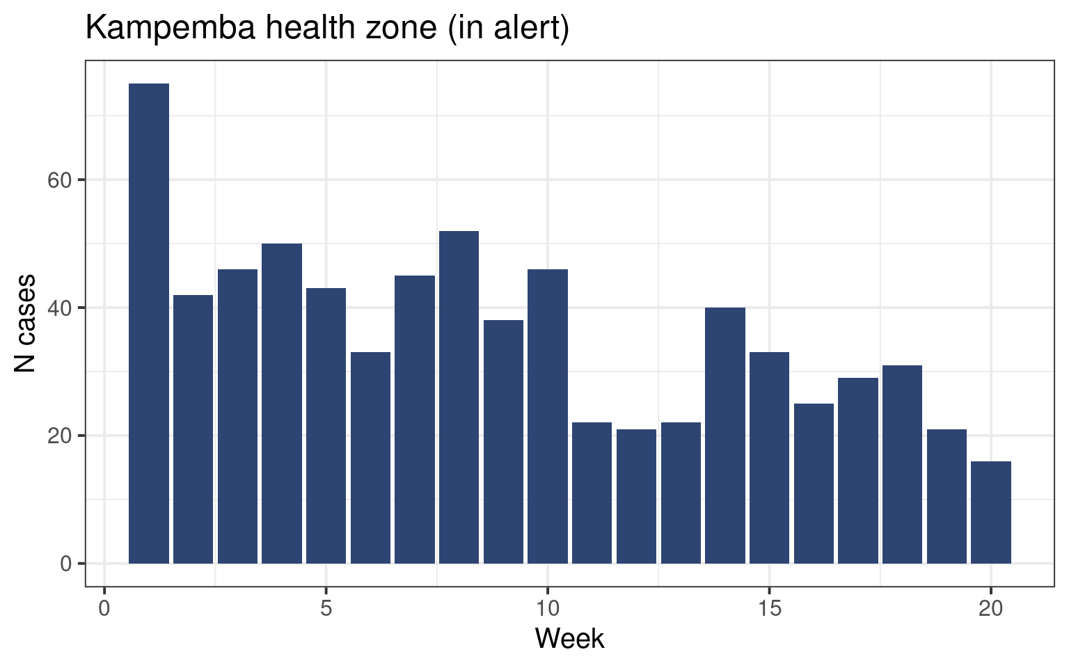
Let us draw the epicurves of health zones currently in alert (in alert during week 20).

We have drawn very similar curves in the epicurve session. Here again we will use the ggplot() function with the geom_col() geom to create a barplot showing the distribution of cases. Since we already have the number of cases per week we do not need to count it ourselved like we did in the past.

Draw an epicurve for one of the health zones in alert.

The graph should look like this (but maybe for another health zone):

The facet_wrap() function allows us to plot several subplots in the same graph (see the faceting satellite for more information on faceting):

data_alert |>
  filter(health_zone %in% hz_alert) |>
  ggplot(aes(x = week, 
             y = totalcases)) + 
  geom_col(fill = "#2E4573") + 
  theme_bw(base_size = 15) + 
  labs(x = "Week",
       y = "N cases",
       title = "Health zones in alert") +
  facet_wrap(vars(health_zone))   # One graph by health_zone

Key indicators (Question 6)

Let’s gather more data on both alerts to help you decide which one to investigate.

Tip

This session builds on summarizing skills seen in the summary session. Do not hesitate to check it or your code if you forgot something.

Week of the first alert

Use the summarize() function to display the first week the alert was raised for each health zone in alert. Which health zone started first?

Surveillance data indicators

Let us go back to the full surveillance dataset that contains more columns of interest.

Add a column cunder_5 to data_surv that contains the the number of cases less than five years.
Derive, for each health zone in alert, the following indicators (organized in a single table):

The number of cases
The number of deaths
The number of less than five year olds
The CFR in percentage
The percentage of reported cases under five

The result should look like this:

  health_zone n_cases n_deaths n_under_5 p_under_5     cfr
1    kampemba     730        0       544 0.7452055 0.00000
2      lwamba     256        2       233 0.9101562 0.78125

Lab data indicators

Now we are going to use the laboratory data to derive a couple more indicators.

For each health zone in alert, derive the following indicators within one table:

The number of patients tested for measles
The number of positives for measles
The percentage of positives for measles
The number of patients tested for rubella
The number of positive for rubella
The percentage of positive for rubella

The result should look like this:

  health_zone n_test_meas n_test_meas_pos positivity_measles n_test_rub
1      lwamba          10               5          0.5000000         10
2    kampemba          14               4          0.2857143         14
  n_test_rub_pos positivity_rubella
1              0         0.00000000
2              1         0.07142857

Tip

Check out the section on summaries with conditions to remind you of the more advanced summaries.

Done!

Congratulation, you are done!

Going Further

Exploring the `complete()` function

Look at the simplified example below: the Kitenge health zone has no row for week 2:

# Create simplified data frame for the example, with three weeks
example_df = data.frame(
  province    = c("haut_katanga", "haut_katanga", "haut_katanga", "haut_lomami", "haut_lomami"),
  health_zone = c("likasi", "likasi", "likasi", "kitenge", "kitenge"),
  week        = c(1, 2, 3, 1, 3),
  totalcases  = c(2, 1, 3, 1, 2))

example_df

      province health_zone week totalcases
1 haut_katanga      likasi    1          2
2 haut_katanga      likasi    2          1
3 haut_katanga      likasi    3          3
4  haut_lomami     kitenge    1          1
5  haut_lomami     kitenge    3          2

We use the following code to make sure that all the health zones have all the possible week values. Since the weeks range from one to three in that toy example, we pass a vector with weeks ranging from one to three:

# Complete the missing week in Kitenge
example_df |> 
  complete(
    nesting(province, health_zone), 
    week = seq(1, 3),             # vector from 1 to 3
    fill = list(totalcases = 0)   # fill new lines with zero (default is NA)
  )

# A tibble: 6 × 4
  province     health_zone  week totalcases
  <chr>        <chr>       <dbl>      <dbl>
1 haut_katanga likasi          1          2
2 haut_katanga likasi          2          1
3 haut_katanga likasi          3          3
4 haut_lomami  kitenge         1          1
5 haut_lomami  kitenge         2          0
6 haut_lomami  kitenge         3          2

Now both health zones within provinces have values for all three weeks.

You may be wondering why we used nesting(province, health_zone) and not just health_zone. The reason is that there could be two health zones in different provinces with the same name. So we need to keep the province column into account. The nesting() argument tells the function to only use the existing combinations of the two columns in the data frame.

Note

If we were passing both column names to the complete() function, it would try to cross all levels of province to all levels of health_zone, which does not make sense in this case:

# Complete the missing week in kikula
example_df |> 
  complete(
    province, health_zone, 
    week = seq(1, 3),  # vector from 1 to 3
    fill = list(totalcases = 0)
  )

# A tibble: 12 × 4
   province     health_zone  week totalcases
   <chr>        <chr>       <dbl>      <dbl>
 1 haut_katanga kitenge         1          0
 2 haut_katanga kitenge         2          0
 3 haut_katanga kitenge         3          0
 4 haut_katanga likasi          1          2
 5 haut_katanga likasi          2          1
 6 haut_katanga likasi          3          3
 7 haut_lomami  kitenge         1          1
 8 haut_lomami  kitenge         2          0
 9 haut_lomami  kitenge         3          2
10 haut_lomami  likasi          1          0
11 haut_lomami  likasi          2          0
12 haut_lomami  likasi          3          0

It would be good to automatically pick the week series, since the data frame is going to change every week. To do that, we can remplace hardcoded values by the smallest and largest week number in the week column to get the range of weeks in the dataset:

# Complete the missing week in kikula
example_df |> 
  complete(
    nesting(province, health_zone),
    week = seq(min(week, na.rm = TRUE),   # vector ranging from smallest to largest week numbers in dataset
               max(week, na.rm = TRUE)),
    fill = list(totalcases = 0)
  )

# A tibble: 6 × 4
  province     health_zone  week totalcases
  <chr>        <chr>       <dbl>      <dbl>
1 haut_katanga likasi          1          2
2 haut_katanga likasi          2          1
3 haut_katanga likasi          3          3
4 haut_lomami  kitenge         1          1
5 haut_lomami  kitenge         2          0
6 haut_lomami  kitenge         3          2

Exploring the `rollaply()` function

If we want to do a cumulative sum of cases over three weeks, we want to apply the sum() function over windows of three weeks.

example_vect <- rep(1, time = 10)
example_vect

 [1] 1 1 1 1 1 1 1 1 1 1

rollapply(
  data  = example_vect,
  width = 3,       # Width of the window  
  FUN   = sum,     # Function to apply, here the sum   
  align = "right"  # Value at row i is the sum of i, i-1 and i-2.
)

[1] 3 3 3 3 3 3 3 3

We inputed a vector of ten values and obtained a vector of lenght height, containing the sums. Obviously the function has a way of dealing with the extremities, and the size of the output is smaller than the size of the input. This would be a problem in a mutate() that creates new columns in a data frame, that need to be the same length as the existing columns.

You can control the behavior at the extremities:

Fill with NA when there is not enough values to calculate a window of three
Allow partial sums (some values represent less than three weeks)

The argument fill = NA pads the extremities with NA (on the left in our case, since we aligned right):

rollapply(
  data  = example_vect,
  width = 3,       # Width of the window  
  FUN   = sum,     # Function to apply, here the sum   
  align = "right", # Windows are aligned to the right
  fill  = NA
)

 [1] NA NA  3  3  3  3  3  3  3  3

It is a reasonnable way of dealing with incomplete windows. In our case however, we can do better: if there were 40 cases in week 1 it would be a cause for alert! We thus want the cumulative sum to be calculated from week one to be able to detect early alerts. The partial = TRUE argument allows this:

rollapply(
  data    = example_vect,
  width   = 3,       # Width of the window  
  FUN     = sum,     # Function to apply, here the sum   
  align   = "right", # Windows are aligned to the right
  partial = TRUE)

 [1] 1 2 3 3 3 3 3 3 3 3

This is close to what we need.

Note

Keeping in mind that since the first two weeks have only partial data compared to later weeks, a lack of alert in these weeks does not necessarily means there is no alert, just that we do not have the data to detect it.

You may remember that arithmetic operations in R return NA if some of the values are NA and we usually need to pass the argument na.rm = TRUE to the functions for them to ignore missing values.

If we had a slightly less complete vector we would have a problem:

example_vect_missing <- c(1, 1, 1, NA, 1, 1)

rollapply(
  data  = example_vect_missing,
  width = 3,       # Width of the window  
  FUN   = sum,     # Function to apply, here the sum   
  align = "right", # Windows are aligned to the right
  partial = TRUE   # Allows sum to be made even if window is less than three
)

[1]  1  2  3 NA NA NA

Fortunately we can pass the na.rm = TRUE argument to rollapply() so that it passes it to sum().

rollapply(
  data  = example_vect_missing,
  width = 3,       # Width of the window  
  FUN   = sum,     # Function to apply, here the sum   
  align = "right", # Windows are aligned to the right
  partial = TRUE,  # Allows sum to be made even if window is less than three
  na.rm = TRUE     # Extra unamed argument to be passed to the sum function
)

[1] 1 2 3 2 2 2

Tip

Here we applied the sum() function to create a cumulative sum over 3 weeks. But you could, with minimal modifications, apply the mean() function to caclulate a moving average!

A last point on the align argument. It defines the position of the rolling windows compared to the value being calculated. The default is that the window is centered: the value i is the sum of values i, i-1 and i+1.

Example of the three alignements (pading with NA to better see what’s happening):

rollapply(data  = c(5, 10, 1, 2, 5, 10),
          width = 3, 
          FUN   = sum,
          align = "left",
          fill = NA)

[1] 16 13  8 17 NA NA

rollapply(data  = c(5, 10, 1, 2, 5, 10),
          width = 3, 
          FUN   = sum,
          align = "center",
          fill = NA)  # The default

[1] NA 16 13  8 17 NA

rollapply(data  = c(5, 10, 1, 2, 5, 10),
          width = 3, 
          FUN   = sum,
          align = "right",
          fill = NA)

[1] NA NA 16 13  8 17

In our case we want the value for a given week to reflect this week and the week past, so we align the window right, to calculate backward in time (by opposition, if we aligned left we would calculate forwards in time).

Nicely formatted percentages

The percent function from the {scales} packages can add percentage formatting to a value.

scales::percent(0.8556)

It takes an accuracy arguments that controls the number of decimals:

scales::percent(0.8556,
                accuracy = 0.1)

You can wrap it around the values that you calulate in the summary tables to change the proportions into nicely formatted percentages.

Important

Once you aplied that function the column is treated as text (since we added a % sign) and you will not be able to do further arithmetical operations on it.

Objectives

Introduction

Setup (Question 2)

Setup a new project

Import data in R

Cleaning (Question 2 and 3)

Surveillance data (Q2)

Quick checks

Clean strings

Save the clean data

Laboratory data (Q2)

Quick checks

Clean and recode strings

Save the clean data

Going further

Complete surveillance dataset (Q3)

Going further

Defining alerts (Question 4)

Preparing the dataset

Subset health zone

Weekly indicator

Cumulative indicator

Cumulative sum

By health zone

Health zones in alert

Draw the epicurve (Question 4)

Key indicators (Question 6)

Week of the first alert

Surveillance data indicators

Lab data indicators

Done!

Going Further

Exploring the complete() function

Exploring the rollaply() function

Nicely formatted percentages

Exploring the `complete()` function

Exploring the `rollaply()` function