Data Importation
Objectives
- Create a RStudio Project
- Set up an organized and well documented code
- Install and load packages
- Write robust file paths
- Import and inspect data
The principles you learned in the Introduction to R session will apply here as well: we should do our best to ensure that our projects won’t just work today but can also be reused and shared in the future. While doing this is not always easy, there are several best practices that can help us, and one of the most important is to start with a good, organized code base.
Setting up your Project
Folder Structure
If not done already, download and unzip the course folder. Save the uncompressed folder to a location that is not connected to OneDrive and navigate into it.
This folder gives an example of a typical (and highly recommended) structure for your code projects:
- 📁 data
- 📁 clean
- 📁 raw
- 📁 R
- 📁 outputs
This folder will be you working directory for all the sessions of this course. You will create an Rstudio project in it (explanations below), and save all your scripts in /R. The course datasets are already in data/raw.
Definitions
To work through this session you need to understand the two following concepts:
Working directory. The working directory is the location (folder) where your R session is actively working. If you save a file, for example, it will be saved into this folder by default. Similarly, when you want to open a file, this folder will be shown by default. All relative paths will be relative to this working directory. By default, R usually picks the “Documents” folder as the working directory on Windows machines.
Root. The root refers to the top-most folder level of the working directory. If your course folder was called FETCHR, the root would then be directly inside it (as opposed to being inside one of its subfolders like R or Data).
RStudio Projects
An RStudio Project can be used to make your life easier and help orient RStudio around the various files used in your code
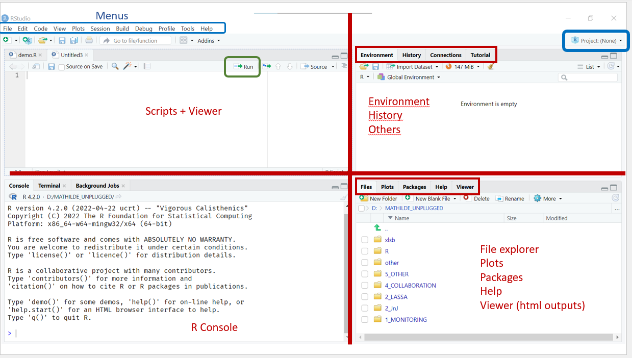
As a quick reminder, your interface should look something like this:

Open RStudio and create a new project by clicking File > New Project > Existing Directory > Browse, navigating into (opening) the course folder, and clicking Create Project.
In the Windows Explorer, look at the course folder. You should now see a new file with the extention .Rproj that has a small blue icon with an R in it.

If you don’t see this file, it’s probably because it is hidden by default on your computer. To change this setting in Windows Explorer, go into the View menu and select Filename Extensions.
When you open an RStudio Project, RStudio starts a new R session, opens the associated project files, and sets your working directory to the root of the course folder. At this time, RStudio also displays the subfolders of this directory in the panel on the bottom right.
It is strongly recommended to set up a separate RStudio Project for each of your analyses to ensure that your project files remain organized and manageable.
There are several ways to open an RStudio Project:
- Use the RStudio menu
File > Open Projectand then select the relevant.Rprojfile - Click on the
Project: (none)button on the top right of the RStudio interface - Navigate in the folder explorer to the analysis folder and double click on the file with the
.Rprojextension
RStudio Options
Before continuing, let’s update some of RStudio’s problematic default settings:
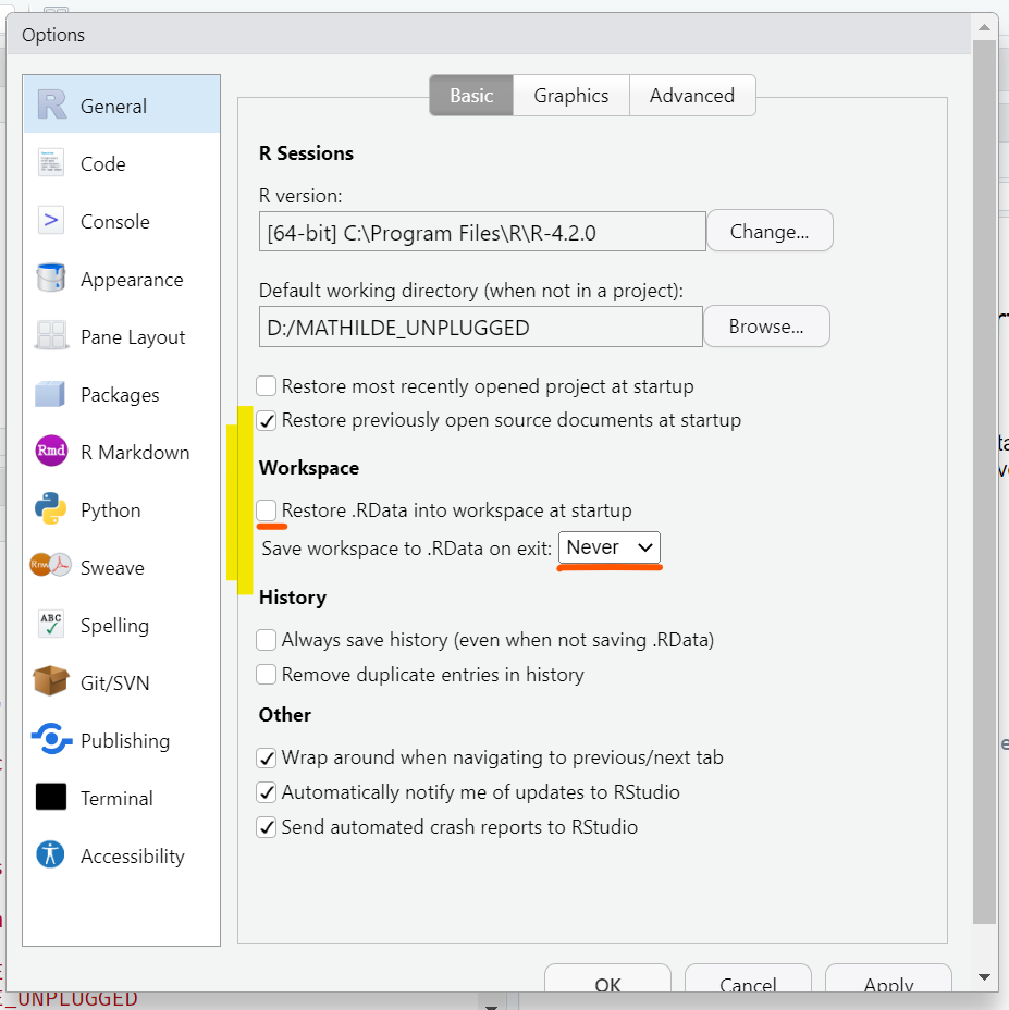
Open the global options (Tools > Global Options) and open the tab General (left menu). Make sure that none of the boxes in the sections R Sessions, Workspace, or History are checked.

When checked, these options cause RStudio to save the objects in your environment and reload them as well as any files you previously had open when you open a new R session. While these default may seem like a good idea, it is better to always start your work from a fresh, empty R session to avoid bugs.
Remember that any commands or outputs that is needed for the cleaning and analysis should be saved explicitly in a script in the correct, functional order.
Creating a New Script
Open a new script and save it in the R folder of your project under the name import_data.R.
Add some metadata to the top of the script as seen in the first session using comments. Be sure to include:
- Title
- Author
- Creation Date
- Description
Now you’re ready to start coding!
Packages
Packages are collections of functions that extend the functionality of R. You’ll use them a lot, both in this course and in your daily life. Fortunately, as an open source language, R packages can be downloaded and installed for free from the internet.
In R, packages are referenced using {}. For example {ggplot2} is the name of the ggplot2 package that contains new plotting functions such as ggplot(), geom_point() etc…
Installation
We can install a new package using the function install.packages(), which downloads and installs it into the package library on your computer. This is done once per computer.
install.packages("here") # install the {here} packageDon’t forget to wrap the package name in quotation marks when using install.packages(). What happens if you don’t do this?
If you are following this session as part of a course, to avoid any potential internet connectivity issues during the training we already had you install most of the course packages.
If are following this tutorial on your own or have not installed the packages yet, you will have to manually install each new package that we encounter.
Usage
Once a package is installed we can use it but we have to specify to R that we will be using it every single session. This process is called loading the package and is achieved using the function library().
library(here) # load the "here" packageUse the library() function to load the packages here and rio, which will be used in the next section.
Based on your computer’s set up and the package you are trying to load, you may get a warning message noting that some functions have been masked or that the current version of the package was built for a different version of R. These messages are not usually a problem but are still important to note.
Try to run the following code. Can you work out what the error means?
library(ggplot)The above code throws an error because you have asked for a library that doesn’t exist. Remember that R is fickle and case sensitive and many of your errors will come from small typos in the names of functions or objects. Here, for example, we wanted to load the package ggplot2 but wrote ggplot instead.
Most of the time, you’ll need to load a number of packages for your script and it is recommended to have a section at the start of your code that loads everything you’ll need in one place:
# Packages ----------------------------
library(tidyverse)   # data manipulation
library(lubridate)   # date manipulation
This practice makes it easy to tell which packages need to be installed to run a script.
Use comments to create a “Packages” section to your script.
Updating Packages
R has a very active community of developers and it’s pretty common for packages to be updated from time to time as their owners add in new functions and fix existing bugs. In order to update the packages in your library, you can go into the Packages tab of the bottom right panel and click Update. Don’t forget that you’ll need to be connected to the internet during this process.
Sometimes packages are updated in a way that might remove or change a function that you used in some of your scripts, causing your code to no longer work. Don’t panic if this happens. The best practice is to adapt your code, although in the worst case scenario you can forcibly install an old version of a package. This is however out of the scope of this session.
Data Importation
Understanding File Paths
To open a file in R you need to provide a file path. A file path is simply a longer name for a file, that includes not only its name but also its location on your computer. There are several ways of defining these paths, including absolute and relative paths.
Absolute Paths
Absolute paths are specific to your computer and go all the way up to the level of your hard drive. For example, an absolute path may look something like this: D:/OneDrive - MSF/Documents/monitoring/cholera/fancy_project/data/raw/example_linelist.xlsx. Clearly, this path will only work on one specific computer.
The use of hard coded absolute paths is strongly discouraged as it makes your code inflexible and prone to break: the paths need to be updated every time your code is shared or the project folder is moved on your computer.
Relative Paths
Relative paths are defined relatively to your current working directory. For example, keeping in mind that our handy .Rproj file set our working directory to the root of our project folder, we could create a relative path that looked like data/raw/example_linelist.xlsx. This means that as long as we maintain the internal structure of our project folder and have an .Rproj file, our code would theoretically run on multiple computers.
Robust Paths with the here() function
The {here} package has a here() function that really helps defining paths. It has two advantages:
- When used with RStudio projects, you can give it only the part of the path within the project, (the relative path in other words), and the function uses it to create the absolute path dynamically.
- It does so using the separator adapted to you operating system, whether it’s
/,\, or//
library(here)
here("data", "raw", "example_linelist.xlsx")
[1] "/tmp/RtmpRJBDYU/file78043d9d3c3c/data/raw/example_linelist.xlsx"See how we only defined the relative path and the function created an absolute path. This way of defining the path will work on your colleagues computer, even if they run on another operating system, as long as you both respect the internal structure of the working directory.
We strongly encourage you to use here() whenever you need to create a file path.
Run the above code in the console. What file path does here("data", "raw") give you?
Using here(), create a complete file path for the file moissala_linelist_EN.xlsx. Keep this path around, we will use it soon.
here() simply creates a file path, it doesn’t actually check if a file exists on your computer: if the file is absent or there is a typo in your code, the command will yield an error when the path is used. If you would like to use a function to check if a file exists, check out the file.exists() function.
We will often want to source multiple data files in a single project. To make that process easier, it can be helpful to create a section at the start of the script, after loading the packages to define paths and store them in variables.
Import function
In R different file formats are often imported using different, often specialized functions. This can be tedious as it requires you to memorize and load a large number of functions just to get your data imported. To avoid this problem, we recommend that you use the import() function from the package {rio}. This function is able to open a large variety of files (including Excel, csv, Stata, and many others) by recognizing the file extension of your data and calling a relevant specialized function from another package so that you don’t have to.
Because import() is actually just calling other functions in the background, it is possible that it will need different arguments depending on the type of file you want to load.
To see the full list of all the file types you can load (and save!) with rio, check out the list of supported formats on their website. In the rest of the lesson we will focus on importing data from Excel .xlsx files.
Importing from the First Sheet
In general, the usage of import() is pretty simple, at minima you need to pass the path of the file to the file argument
import(file = here("data", "raw", "example_linelist.xlsx"))Notice that we have nested the command here() inside the import() command. Nesting functions is absolutely allowed in R and is something you will do all the time. When functions are nested, R will evaluate them in the order of the innermost function (in this case here()) to the outermost (in this case import()). In this way, the output of here() is being used as the input of import().
Import the file moissala_linelist_EN.xlsx that is in your raw data subfolder into R using here() and import().
If your import worked correctly, R will print the data into the console but not save it into the environment because we have not assigned them to an object.
You may not want to have R print very large datasets into the console and assign them directly to an object.
Reimport your data but this time save it to an object called df_linelist.
Importing Data from Any Sheet
As you just saw, R selects the first sheet by default. It is however possible to pass the number (or name) of a specific worksheet in your Excel data to import() using the argument which:
import(file = here("data", "raw", "example_linelist.xlsx"),
       which = 2)  # imports the second sheet
Note that the which argument is specific to the file types that have multiple sheets, such as Excel or .Rdata files. If you try to use it on a .csv file the argument will be ignored.
Taking a First Look at your Data
We have now imported a dataset into R and assigned it to a dataframe (df_linelist). The natural next step is to inspect this dataset, to check that the import went well, get to know it a bit better, and assess if it requires any cleaning before analysis.
We can start by taking a quick look at the first few lines of the dataframe using the function head(). This function takes a dataframe as its first argument and optionally accepts a second argument n indicating the number of lines we would like to see.
head(df_linelist, n = 10) # Inspect 10 first linesUse head() to examine the 12 first lines of df_linelist.
We can also check out our data by looking at the Environment tab of the top-right panel. Here, we can see our dataframe in the environment, look at its structure, or open it in the data viewer of RStudio.
Click on the round blue button next to df_linelist in your environment to see its structure. Then click on the name of the dataset to open it in the viewer.
The data viewer displays dataframes as tables and is a convenient way to quickly look at your data. You can even sort and filter your data in the “View”, though be aware that these actions will not make any changes to the actual object df_linelist. The View can also be opened by passing the dataframe to the function View().
Done!
Well done and don’t forget to save your code.
Going Further
Extra Exercises
- Use
dim()to take a look at the dimensions of your dataset. - Use
str()to check the data type of each column. Does anything look odd? Remember that you can also use functions likeis.character()andis.numeric()if you’d like to test the type of a particular column. - Using a function learned in the first session, can you extract the names of the columns of the dataset? Do these results match what you see when you open the data in Excel?
- Try passing your dataframe to the function
summary(). What does this function tell you?
Additional Resources
- The
{rio}website - More examples on importing data of various file types